How to Use INDEX and MATCH in Excel – Step-by-Step Guide

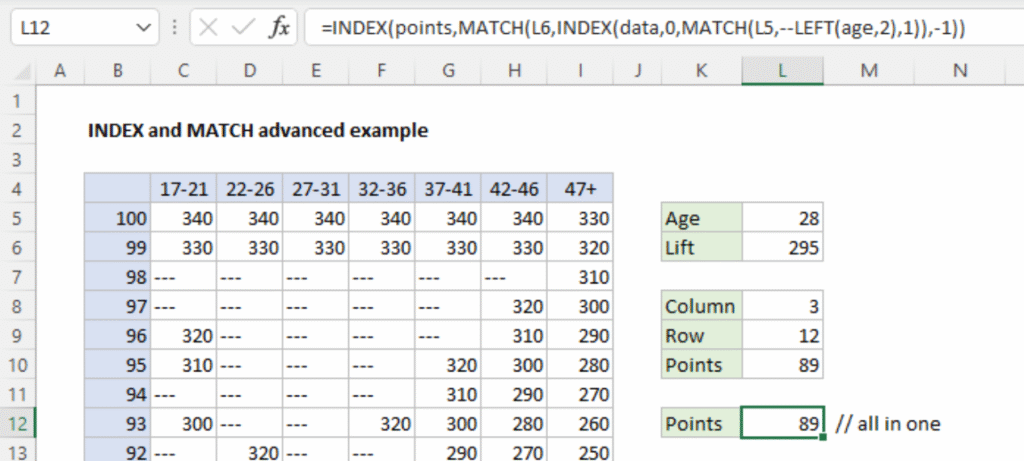
Imagine you have a giant table of data in Excel and you need to find one specific piece of information—say, the price of “Widget B” in March—without manually scanning through rows and columns.

That’s where the powerful duo of INDEX and MATCH comes in. Together, they let you look up values anywhere in your sheet, faster and more reliably than many other methods.

In this guide, we’ll break down exactly how each function works on its own, and then show you step by step how to combine them into a single, flexible lookup tool. No jargon, no fluff—just clear, simple instructions so even a fifth-grader can master them!

Table of Contents

What Are `INDEX` and `MATCH`?

INDEX: Picks out a value from a specific row and column within a given range.
MATCH: Finds the position of a given value within a row or column.

Alone, they’re helpful; together, they form a lookup powerhouse.

Must Read: How to Track Expenses Using Excel: Complete Guide for Personal Finance Management

Why Use `INDEX` + `MATCH` Instead of `VLOOKUP`?

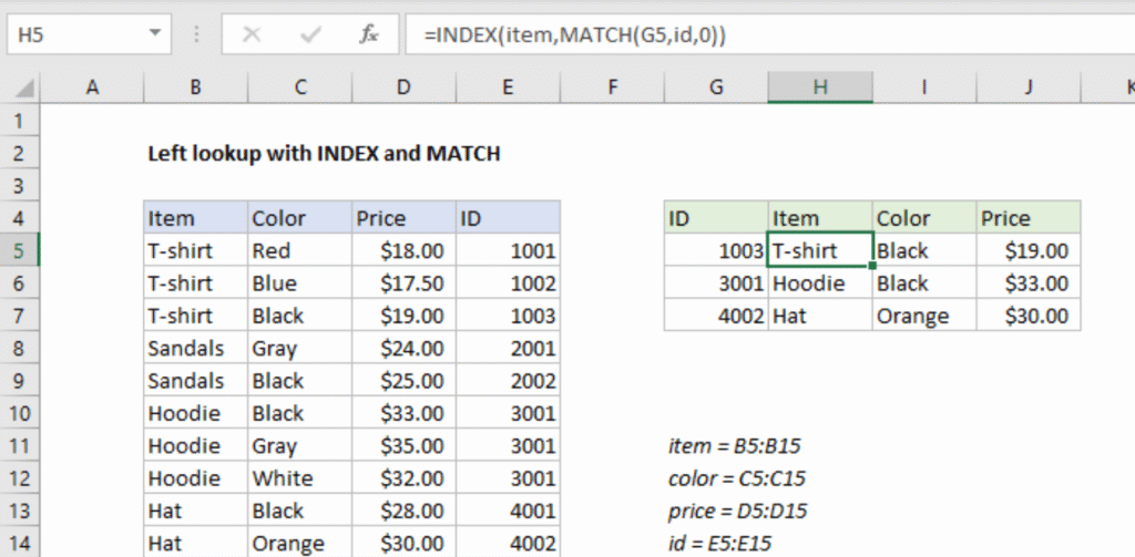
Left-Side Lookups
- VLOOKUP only searches the leftmost column.
- INDEX+MATCH can look anywhere.
Speed & Efficiency
- Recalculates faster on large datasets.
Resilient to Column Changes
- Won’t break if you insert or delete columns.

How the `INDEX` Function Works

excelCopyEdit=INDEX(array, row_number, [column_number])

array: Range to pull from.
row_number: Which row in that range.
column_number: Which column (optional if single column).

Example:
To get Bob’s score (92) from B2:B4:

excelCopyEdit=INDEX(B2:B4, 2)

How the `MATCH` Function Works

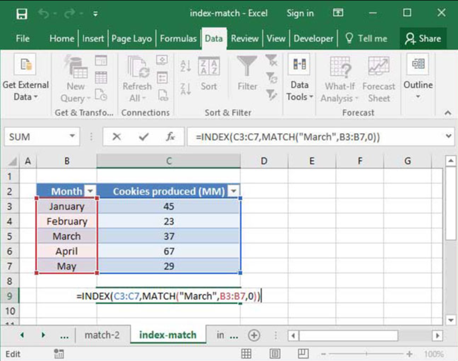
excelCopyEdit=MATCH(lookup_value, lookup_array, match_type)

lookup_value: What to find.
lookup_array: The row/column to search.
match_type: Use 0 for exact match.

Example:
To find Bob in A2:A4:

excelCopyEdit=MATCH("Bob", A2:A4, 0)

Returns 2.

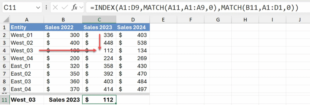
Putting `INDEX` and `MATCH` Together

excelCopyEdit=INDEX(
  return_range,
  MATCH(row_lookup, row_range, 0),
  MATCH(col_lookup, col_range, 0)
)

First MATCH → row number.
Second MATCH → column number.
INDEX pulls the intersection.

Step-by-Step Walkthrough with an Example

Table:

	A	B	C	D
1	Product	Jan Price	Feb Price	Mar Price
2	Widget A	10	12	11
3	Widget B	15	14	16
4	Widget C	8	9	10

Goal: Find “Widget B” price in March.

Define ranges
- return_range = B2:D4
- row_range = A2:A4
- col_range = B1:D1
Formula excelCopyEdit=INDEX( B2:D4, MATCH("Widget B", A2:A4, 0), MATCH("Mar Price", B1:D1, 0) )
Results
- Row match → 2
- Column match → 3
- INDEX(B2:D4, 2, 3) → 16

Must Read: What Are Some Time-Saving Tips for Excel? 25 Expert Strategies to Boost Your Productivity

How to use INDEX match for 2 criteria?

Create a helper column that joins the two criteria, or use an array formula:

excelCopyEdit=INDEX(return_range,
  MATCH(1, (criteria1_range=criteria1)*(criteria2_range=criteria2), 0)
)

(In older Excel, confirm with Ctrl + Shift + Enter.)

How to use VLOOKUP and INDEX match together?

You can use VLOOKUP to return an array of values, then INDEX to pick one:

excelCopyEdit=INDEX(
  VLOOKUP(key, table, {2,3,4}, FALSE),
  1,   /* row within returned array */
  2    /* column within returned array */
)

How do you use the INDEX in Excel?

Single column: =INDEX(A2:A10, 4) returns the 4th item.
Two-dimensional: =INDEX(A2:D10, 3, 2) returns the cell at row 3, column 2.

Why do people use INDEX match?

To look left of the key column.
To build two-way or multi-criteria lookups.
For speed and stability in large workbooks.

Common Mistakes to Watch For

Omitting 0 in MATCH → wrong matches.
Mismatched ranges → formula errors.
Typos/spaces in lookup values → use TRIM().
Not locking ranges when copying → use absolute references ($A$2:$A$4).

Handy Tips and Tricks

Wildcards: MATCH("*"&value&"*", range, 0) for partial text.
Two-way lookups: As shown above, combine two MATCH calls.
Error handling: IFERROR(..., "Not found").

Conclusion

The INDEX + MATCH combination is a versatile, reliable, and efficient way to perform lookups in Excel. Unlike VLOOKUP, it doesn’t care about column order, and it handles large datasets with ease.

Once you’ve mastered the simple steps—identifying your ranges, writing the two MATCH functions, and wrapping them in INDEX—you’ll wonder how you ever managed without it. Practice with your own data, and soon you’ll be using these functions without thinking twice!