How to Filter & Sort Data Effectively in Excel – Step‑by‑Step Guide

Filtering and sorting data are two of the most powerful and commonly used features in Microsoft Excel. Whether you’re tracking your allowance, organizing your book list, or managing large sets of sales numbers at work, learning how to filter and sort will make your life easier.

In this guide, we’ll walk through everything you need to know to filter and sort data effectively in Excel, step by step. We’ll use simple language and clear examples so that even a fifth grader can follow along.

Let’s get started!

Must Read: Why Is Excel Not Calculating Formulas? 9 Simple Fixes to Resolve It

What Is Sorting?

Sorting means rearranging the rows of your data so that the values in one column go from smallest to largest (ascending) or largest to smallest (descending). You can sort numbers, dates, or text (like names or places).

• Ascending sort: 1, 2, 3, … or A, B, C, … or January, February, March, …
• Descending sort: 3, 2, 1, … or Z, Y, X, … or December, November, October, …

Sorting is useful when you want to see the biggest or smallest things first. For example, you might sort test scores to see who scored highest, or sort dates to find the earliest event.

What Is Filtering?

Filtering means hiding the rows you don’t want to see, so you only show the rows that meet certain rules. For example:

• Show only students who scored above 90.
• Show only events happening in July.
• Show only items that cost more than $50.

After you apply a filter, all of the other rows are hidden until you clear the filter. This makes it easy to focus on a subset of your data.

How to Sort Data in Excel

1. Select Your Data

1. Click any cell in the column you want to sort.
2. Or click and drag to highlight the exact range of cells (including all the rows you want sorted).

2. Sort with the Ribbon Buttons

1. Go to the Home tab on the ribbon.
2. Look for the Sort & Filter group on the right.
3. Click Sort A to Z for an ascending sort (smallest to largest or A→Z).
4. Click Sort Z to A for a descending sort (largest to smallest or Z→A).

Excel will automatically detect the rest of the data in that row and move entire rows so that your chosen column ends up sorted.

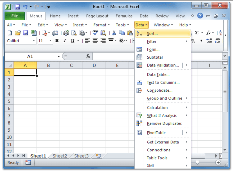
3. Custom Sort Dialog Box

If you need more control, use the Custom Sort dialog:

1. Click Sort (instead of the A→Z or Z→A buttons).
2. In the dialog box, under Column, pick which column you want to sort by.
3. Under Sort On, choose Values, Cell Color, Font Color, or Cell Icon.
4. Under Order, pick A to Z, Z to A, Smallest to Largest, or Largest to Smallest (depending on your data).
5. Click Add Level to sort by more than one column (e.g., sort by Class, then by Name within each class).
6. Click OK to apply.

How to Filter Data in Excel

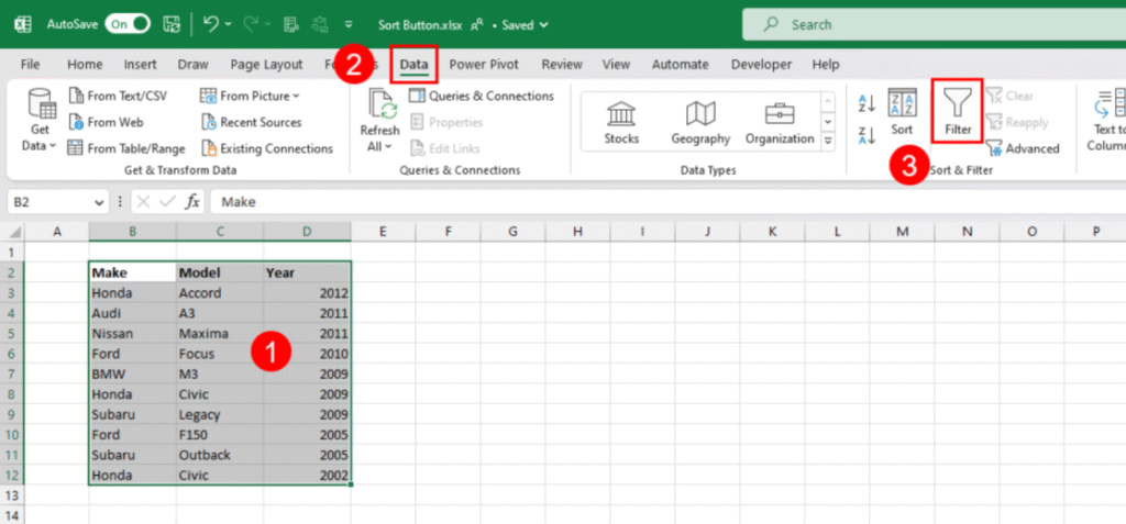
1. Turn on Filtering

1. Click any cell in your data range.
2. Go to the Home tab (or Data tab).
3. Click Sort & Filter → Filter.
4. Tiny drop‑down arrows appear in each header cell (the first row).

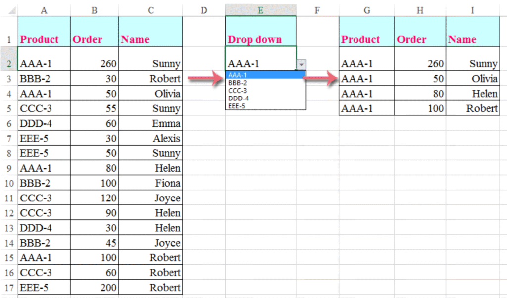
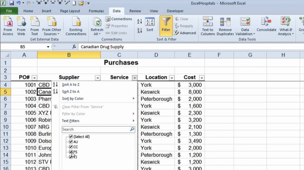
2. Apply a Basic Filter

1. Click the drop‑down arrow in the column you want to filter.
2. Uncheck Select All.
3. Check the box next to the value(s) you want to keep.
4. Click OK.

Only rows with the checked values will remain visible. All other rows are hidden.

3. Use Number, Text, or Date Filters

In the drop‑down menu, you can choose from special filters:

• Number Filters: Greater Than, Less Than, Between, Top 10, etc.
• Text Filters: Begins With, Ends With, Contains, Custom Filter, etc.
• Date Filters: Before, After, Between, This Month, Next Quarter, etc.

For example, to show only sales above $1,000:

1. On the Sales column drop‑down, choose Number Filters → Greater Than…
2. Enter 1000.
3. Click OK.

Combining Sorting and Filtering

Filtering and sorting work together. You can filter your data first to hide unwanted rows, and then sort the visible rows. Or you can sort first (to order all rows) and then filter (to hide some rows).

Example Workflow

1. Filter to show only “East Region” sales.
2. Sort those filtered rows by “Revenue” descending to see the biggest sales first.

Excel remembers both settings, so you can clear filters or remove sort orders independently.

Multi‑Level Sorting

Sometimes you need to sort by more than one column. For example, sort by Class and then by Name within each class:

1. Click Sort & Filter → Custom Sort.
2. Under Column, pick Class. Under Order, pick A to Z.
3. Click Add Level.
4. Under the new level, pick Name, A to Z.
5. Click OK.

First Excel groups all rows by class in A→Z order, then sorts students within each class alphabetically.

Custom Sort Orders

Excel has built‑in orders (A→Z, Small→Large, etc.), but you can make your own:

1. Go to File → Options → Advanced.
2. Scroll to General and click Edit Custom Lists….
3. Type your list items in order (one per line), e.g., High, Medium, Low.
4. Click Add, then OK.

When you sort, choose Custom List under Order and pick your list. Excel sorts according to that order.

Advanced Filtering

Excel’s Advanced Filter (on the Data tab) lets you:

• Copy filtered results to another sheet.
• Use complex criteria (e.g., “Show rows where Region = East AND Sales > 1000”).
• Filter data in place or to a new location.

Steps

1. Prepare a criteria range: copy your headers and set up criteria below.
2. Click Advanced in the Sort & Filter group.
3. Choose your List range (your data).
4. Choose your Criteria range.
5. Pick Filter the list, in-place or Copy to another location.
6. Click OK.

Tips for Clean Data Before Sorting & Filtering

1. Remove Blank Rows/Columns: Blank rows confuse Excel about where the data ends.
2. Convert to Table: Select your range and press Ctrl+T to make a Table. Tables auto‑expand and have built‑in sort/filter arrows.
3. Ensure Correct Data Types: Dates should be real dates, not text. Numbers should be formatted as numbers.
4. Freeze Headers: Use View → Freeze Panes → Freeze Top Row so you always see your headers.

Common Pitfalls & How to Avoid Them

Problem	Cause	Fix
Headers get sorted with data	“My data has headers” unchecked	In Custom Sort, make sure My data has headers is checked so Excel keeps the header row in place.
Filters disappear after editing data	Data converted outside the table range	Convert your data to a Table (Ctrl+T) so filters automatically adjust when you add or remove rows.
Numbers sorted as text	Numbers stored as text	Convert text to numbers: select column, click the warning icon, choose Convert to Number, or use Data → Text to Columns wizard.
Unexpected rows included/excluded	Blank rows/columns in the range	Remove any blank rows/columns within your data before sorting/filtering.

Best Practices

• Save Before Big Sorts: Make a copy of your sheet in case the sort goes wrong.
• Use Tables: Tables auto‑update filters and sorts when you add new data.
• Name Your Ranges: Named ranges prevent Excel from guessing the wrong data area.
• Document Your Steps: If other people use your file, note which filters/sorts you applied.

Must Read: How to Automate Tasks in Excel: The Complete Guide to Streamline Your Workflow in 2025

Conclusion

Sorting and filtering are essential skills for anyone who works with data in Excel. By learning how to:

• Sort simple and multi‑level lists
• Apply basic and advanced filters
• Combine filters and sorts
• Create custom sort orders
• Keep your data clean and well‑formatted

you’ll save hours of time and reduce mistakes. Practice these steps on your own data, and soon filtering and sorting will feel like second nature!