

Creating a pivot table in Excel is one of the most powerful and time‑saving ways to analyze, summarize, and visualize your data.
With just a few clicks, you can turn hundreds or thousands of rows of data into a concise, interactive report that reveals trends, patterns, and insights at a glance.
In this comprehensive guide, you’ll learn everything you need to know to create, customize, and use pivot tables effectively—even if you’re just in fifth grade!
Read More: Can Excel Help in Personal Budgeting? The Complete Guide for 2025
What Is a Pivot Table?
A pivot table is an interactive Excel tool that lets you:
- Summarize large datasets quickly
- Rearrange (or “pivot”) data to view it from different angles
- Filter and drill down into the details behind the numbers
- Create custom calculations without writing formulas
Think of a pivot table as a smart, self‑service report builder. You drag field names (column headers) into different “buckets” (areas) to instantly generate sums, averages, counts, percentages, and more.
Why Use a Pivot Table?
Pivot tables are popular because they:
- Save Time
- No more manual sorting, filtering, or subtotaling thousands of rows.
- Offer Flexibility
- Change your summary view with a quick drag‑and‑drop.
- Encourage Exploration
- Easily spot trends and outliers by rearranging data.
- Require No Complex Formulas
- Perform calculations like sums, counts, averages, and percentages automatically.
Whether you’re tracking sales by region, analyzing project hours, or reviewing survey results, pivot tables turn data into insights in seconds.
Preparing Your Data
A pivot table works best when your data is well‑organized. Follow these simple rules:
- Use a Table or Range
- Convert your data into an Excel Table (Insert → Table) for automatic expansion as you add rows.
- Have Clear Headers
- Each column should have a unique, descriptive heading in the first row.
- No Blank Rows or Columns
- Gaps can confuse Excel’s data detection and lead to incomplete pivot tables.
- Consistent Data Types
- Dates in one column, numbers in another, text in another—don’t mix types in the same column.
Tip: If your data changes often, turn it into a Table (Ctrl + T). Any new rows will automatically be included in your pivot table when you refresh.
Step‑by‑Step: Inserting a Pivot Table
- Select Your Data Range
- Click any cell within your data range or Excel Table.
- Go to the Ribbon
- Click Insert → PivotTable.
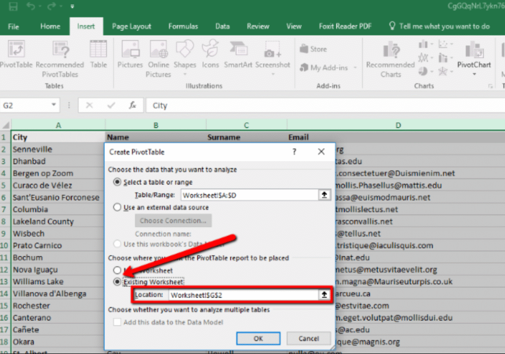
- Choose Your Data Source
- Excel will auto‑select your range or Table name (e.g., Table1).
- Pick a Placement
- New Worksheet (recommended) or Existing Worksheet.
- Click OK
Excel creates an empty pivot table frame and shows the PivotTable Fields pane on the right.
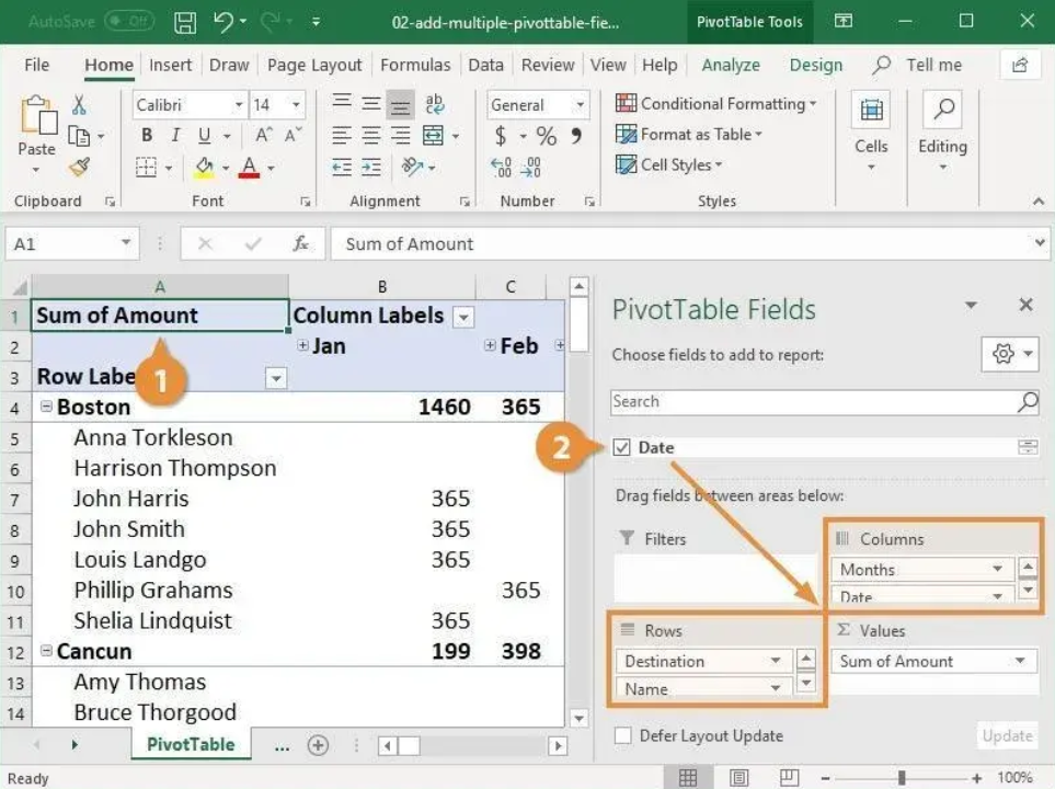
Building Your Pivot Table
You’ll use the PivotTable Fields pane to build your report. It has four areas:
- Filters
- Columns
- Rows
- Values
Drag field names (your column headers) into these areas.
Adding Rows and Columns
- Rows Area
- Fields here become row labels on the left side of the table.
- E.g., drag “Region” to Rows to list each region vertically.
- Columns Area
- Fields here become column labels along the top.
- E.g., drag “Product” to Columns to show each product across the top.
Example:
| Region | Product A | Product B | Product C |
|---|---|---|---|
| North | |||
| South |
Adding Values (Summaries)
- Values Area
- Drag numeric fields here to summarize (Sum, Count, Average, etc.).
- By default, Excel sums numbers and counts text.
- Changing the Calculation
- Click the ▼ next to the field in Values.
- Choose Value Field Settings.
- Pick Sum, Count, Average, Max, Min, % of Grand Total, etc.
Example: If you drag “Sales” to Values, you’ll see total sales by row/column intersection.
Using Filters and Slicers
- Report Filter
- Drag a field (e.g., “Year”) into Filters to show data for a single year at a time.
- Slicers (Excel 2010+)
- Click anywhere in the pivot.
- Go to PivotTable Analyze → Insert Slicer.
- Select a field.
- Click OK.
- Slicers are visual buttons that let you click to filter.
Note: Slicers can also connect to multiple pivot tables for synchronized filtering.
Customizing Your Pivot Table
Excel offers many ways to tweak the look and feel of your pivot table so the data is clear and professional.
Design and Layout Options
- Select any cell in the pivot.
- Go to the Design tab under PivotTable Tools.
- Choose a Report Layout:
- Compact, Outline, or Tabular.
- Pick a PivotTable Style:
- Light, Medium, or Dark color schemes.
- Toggle options like:
- Banded Rows (alternating shading)
- Banded Columns
- Grand Totals and Subtotals
Number Formatting
- In the Values area, click the ▼ next to a field.
- Choose Value Field Settings → Number Format.
- Pick Number, Currency, Percentage, Date, etc.
- Set decimal places, thousand separators, currency symbols.
Tip: Formatting numbers at the pivot level keeps your source data unchanged.
Grouping Data
Dates
- Right‑click any date in the pivot.
- Choose Group….
- Group by Months, Quarters, Years, or even Days.
Numbers
- Right‑click a number field in Rows or Columns.
- Choose Group….
- Define a start, end, and interval (e.g., group ages into 0–10, 11–20, 21–30).
Manual Groups
- Select multiple items (Ctrl+Click) in the pivot.
- Right‑click → Group to create a custom group.
Refreshing and Maintaining Your Pivot Table
Any time the source data changes—new rows added, values updated—you must refresh the pivot table:
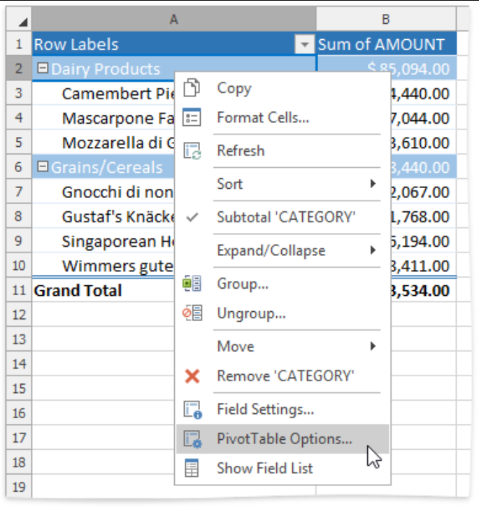
- Single Pivot:
- Right‑click inside the pivot → Refresh.
- Multiple Pivots or Data Model:
- On the Ribbon: Data → Refresh All.
Auto‑Refresh Tip: You can create a simple macro that refreshes all pivots when you open the workbook, but that’s beyond the scope of this guide.
Common Pivot Table Pitfalls (and How to Fix Them)
- Blank Rows/Columns in Source
- Pivot won’t see data past the blank.
- Fix: Remove blanks or convert to Table.
- Incorrect Totals
- Caused by text stored as numbers or vice versa.
- Fix: Clean data types (use VALUE function, Text to Columns).
- Missing Items
- Pivot caches old items even if removed from source.
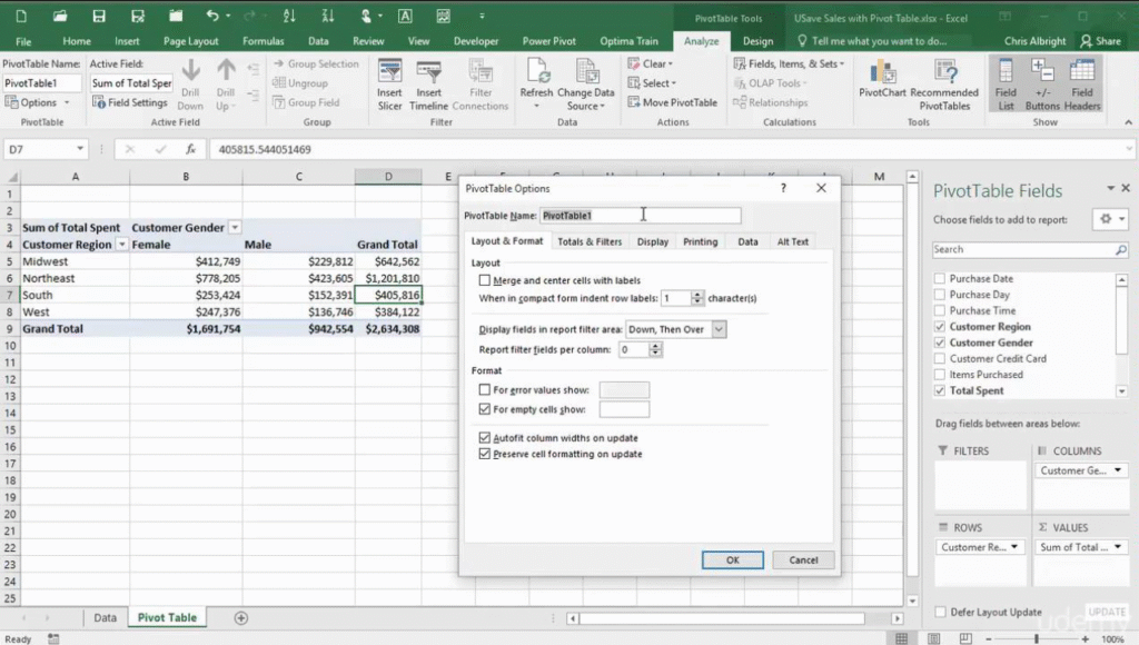
- Fix: In PivotTable Options → Data tab, set Number of items to retain per field to None, then refresh.
- Large File Size
- Pivot cache can bloat file.
- Fix: Clear unused items in PivotTable Options or save as XLSB.
Must Read: How Do Professionals Use Excel at Work: Complete Guide for 2025
What Is the Use of a PivotTable in Excel?
A PivotTable lets you summarize, analyze, and explore large amounts of data in just a few clicks. With a PivotTable you can:
- Quickly aggregate data (sum, count, average, min/max) without writing formulas.
- Rearrange (“pivot”) rows and columns to view your data from different angles.
- Filter and slice your data to focus on specific items or time periods.
- Group dates (months, quarters, years) or numbers into custom bins.
- Drill down into details behind any total or subtotal.
Think of it as a self‑service reporting tool: drag field names into four buckets (Rows, Columns, Values, Filters) and instantly get meaningful summaries.
How Do I Create a PivotTable in Excel with Multiple Data Ranges?
Sometimes your data isn’t all in one table. To create a PivotTable from multiple data ranges:
- Turn Each Range into a Table
- Select each data range → Insert → Table (or press Ctrl + T).
- Give each table a clear name on the Table Design tab (e.g.,
SalesTable,RegionTable).
- Create a Data Model
- Go to Insert → PivotTable.
- In the dialog, check Add this data to the Data Model before clicking OK.
- Add Additional Tables
- With the new PivotTable selected, go to PivotTable Analyze → Fields, Items & Sets → Manage Data Model (Power Pivot window opens).
- In Power Pivot, choose Existing Connections → Tables → Add each of your named tables.
- Create Relationships
- In the Power Pivot window, go to Diagram View.
- Drag the key column (e.g.,
RegionID) from one table onto the matching column in the other table. - This links the tables so you can pull fields from both.
- Build Your PivotTable
- Close Power Pivot. Back in Excel’s PivotTable Fields pane, you’ll now see all tables’ fields.
- Drag fields from each table into Rows, Columns, Values, and Filters just like a single‑table PivotTable.
How to Pivot Step by Step?
Here’s a straightforward 5‑step process to create any PivotTable:
- Prepare Your Data
- Ensure your data has clear column headers, no blank rows/columns, and consistent data types.
- (Optional) Convert your range into a Table via Insert → Table.
- Insert the PivotTable
- Click any cell in your data (or table).
- Go to Insert → PivotTable.
- Confirm the range or table name, choose “New Worksheet,” and click OK.
- Lay Out Your Fields
- In the PivotTable Fields pane, drag:
- Rows: the field you want listed vertically (e.g., Region).
- Columns: the field you want across the top (e.g., Quarter).
- Values: the numeric field you want to summarize (e.g., Sales).
- Filters (optional): a field you want to filter by (e.g., Year).
- In the PivotTable Fields pane, drag:
- Customize Your Calculations
- By default, numeric fields sum and text fields count.
- To change: click the ▼ next to your value field → Value Field Settings → choose Sum, Count, Average, etc.
- Refine and Explore
- Filter using the Filters area or add Slicers via PivotTable Analyze → Insert Slicer.
- Group dates or numbers by right‑clicking a field in the pivot and choosing Group.
- Design the look under Design → PivotTable Styles and Report Layout.
What Is the “Formula” for a PivotTable in Excel?
PivotTables themselves aren’t built with a single worksheet formula—instead they use their own engine. But you can extract specific PivotTable results with the GETPIVOTDATA function.
GETPIVOTDATA syntax:
plaintextCopyEdit=GETPIVOTDATA(
   data_field,   // the name of the value field (e.g., "Sum of Sales")
   pivot_table,  // a reference to any cell in the PivotTable
   [field1, item1],  // one or more pairs of field names and item names
   …
)
Example:
If your PivotTable sums “Sales” by “Region,” and cell B3 in the pivot is the Grand Total of Sales, you could get North region’s total like this:
excelCopyEdit=GETPIVOTDATA(
   "Sum of Sales",
   $B$3,
   "Region", "North"
)
- “Sum of Sales” must exactly match the value field name.
- $B$3 should point to any cell in the PivotTable.
- Then you specify which row or column you want (Region = North).
Tip: To turn GETPIVOTDATA on or off, go to PivotTable Analyze → Options → uncheck/check Generate GetPivotData.
Tips & Tricks for Power Users
- Calculated Fields & Items
- Create custom formulas right in the pivot (PivotTable Analyze → Fields, Items & Sets).
- Show Values As
- Display values as % of Row Total, % of Column Total, Difference From, Running Total, Rank, etc.
- Multiple Consolidation Ranges
- Combine data from multiple sheets or ranges.
- Pivot Charts
- Create dynamic charts linked to your pivot (Insert → PivotChart).
- Get & Transform (Power Query)
- Use Power Query to shape and clean data before pivoting.
Conclusion
Pivot tables are the go‑to tool for anyone who needs to summarize, analyze, and visualize large datasets in Excel.
By following the steps in this guide—preparing your data, inserting a pivot table, building your report, and customizing the layout—you can turn raw numbers into clear, interactive summaries in minutes.
Practice with your own data, explore the grouping and “Show Values As” features, and soon you’ll be an Excel pivot table pro!
