

Freezing panes in Excel is like sticking a label at the top or side of your worksheet so that key information always stays in view—even when you scroll through hundreds or thousands of rows and columns.
Whether you’re organizing your school grades, tracking monthly expenses, or analyzing a large data set, freezing panes helps you keep your headers, labels, or important fields visible at all times.
Must Read: Power Pivot vs Pivot Table: Key Differences & When to Use Each
What Does “Freeze Panes” Mean?
When you freeze panes, Excel locks specific rows or columns so they remain visible no matter how far you scroll. If you freeze the top row, it will stay at the very top of your worksheet even when you scroll down.
If you freeze the first column, it will stay on the left side when you scroll right. You can also freeze both rows and columns at once by selecting a cell below and to the right of the area you want to lock.
Freezing panes is different from splitting panes. Splitting creates adjustable “windows” within the same sheet; freezing simply locks rows or columns in place.
Why Should You Use Freeze Panes?
- Always See Your Headers
In a big table, you don’t want to scroll back up to remember what each column means. Freezing the header row keeps it visible so you always know what you’re looking at. - Compare Data Easily
If you want to compare data from the top of your list with items further down, freezing the header row ensures you never lose track of which column is which. - Stay Oriented in Large Sheets
It’s easy to get lost in a sheet with hundreds of rows. Frozen panes give you a fixed reference point, so you always know where you are. - Increase Productivity
By keeping labels in view, you can work faster and make fewer mistakes when entering or reviewing data.
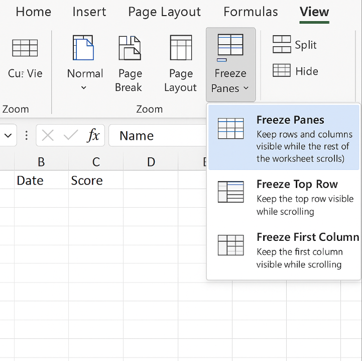
The Three Freeze-Panes Options
Under the View tab on the Ribbon, you’ll find the Freeze Panes button. Click the dropdown arrow to see three options:
- Freeze Panes
Locks every row above and every column to the left of the active cell. - Freeze Top Row
Locks only row 1, regardless of your current cell selection. - Freeze First Column
Locks only column A, regardless of your current cell selection.
How to Freeze Panes: Step‑by‑Step
1. Open Your Worksheet
Make sure you have the Excel file open and are on the correct sheet.
2. Decide What to Freeze
- Just the top row? Use Freeze Top Row.
- Just the first column? Use Freeze First Column.
- Both multiple rows and columns? Select a cell below and to the right of the area you want to lock.
3. Navigate to the View Tab
- Click the View tab on the Ribbon.
- In the Window group, click Freeze Panes.
4. Choose Your Option
- Freeze Panes: Locks rows above and columns to the left of your selected cell.
- Freeze Top Row: Locks only row 1.
- Freeze First Column: Locks only column A.
Excel displays thin, solid lines indicating which panes are frozen.
Detailed Examples
A. Freezing the Top Row
- On any cell, go to View → Freeze Panes → Freeze Top Row.
- Now row 1 stays in view as you scroll down.
Use this when your column headers (like “Date,” “Name,” “Amount”) are in row 1.
B. Freezing the First Column
- Go to View → Freeze Panes → Freeze First Column.
- Column A remains visible when you scroll right.
Use this when your row labels (like “Product ID,” “Student Name”) are in column A.
C. Freezing Multiple Rows and Columns
To freeze the first two rows and the first column:
- Click any cell in row 3 (e.g., A3).
- Go to View → Freeze Panes → Freeze Panes.
Rows 1–2 and column A will be locked in place. Always select one row below and one column to the right of what you want frozen.
How to Unfreeze Panes
When you’re done and no longer need the panes frozen:
- Go to View → Freeze Panes.
- Click Unfreeze Panes.
This restores normal scrolling for all rows and columns.
Keyboard Shortcuts for Freezing Panes
Using the keyboard can speed up your workflow:
- Freeze Panes (rows above and columns left of active cell)
Alt→W→F→F - Freeze Top Row
Alt→W→F→R - Freeze First Column
Alt→W→F→C - Unfreeze Panes
Alt→W→F→U
Practice these shortcuts to become more efficient in Excel.
Troubleshooting Common Issues
- Option Grayed Out
- You might be in Page Layout or Page Break Preview view. Switch to Normal view under View → Workbook Views → Normal.
- Make sure no shapes or charts are selected. Click an empty cell first.
- Can’t Freeze More Than One Row with “Freeze Top Row”
- Use the general Freeze Panes option instead of Freeze Top Row if you need more than one row.
- Sheet Is Protected
- If the sheet is protected, you may need to unprotect it under Review → Unprotect Sheet (password may be required).
- You See Split Bars Instead of Frozen Lines
- You used Split instead of Freeze Panes. Remove the split under View → Split, then freeze correctly.
Pro Tips and Best Practices
- Plan Your Layout: Decide in advance which headers or labels are essential.
- Use Excel Tables: Converting your data range to an official Excel Table (Ctrl + T) keeps headers visible automatically.
- Combine with Filters: Freeze your header row before using filters so you can always see column names.
- Watch Hidden Rows/Columns: Hidden rows or columns above or to the left still count when determining the freeze point.
- Stay in Normal View: Always use Normal view when freezing panes.
Must Read: How to Create a Dynamic Chart in Excel: The Complete 2025 Guide
Frequently Asked Questions
1. What is the shortcut for freezing panes in Excel?
- Alt, then W, F, F to freeze panes.
- Alt + W, F, R to freeze the top row.
- Alt + W, F, C to freeze the first column.
- Alt + W, F, U to unfreeze.
2. How do you lock a line in Excel so it doesn’t move?
Locking a line is the same as freezing a row.
- Click in the row below the one you want locked.
- Press Alt + W, F, F (to freeze both rows and columns based on your selection) or Alt + W, F, R (to freeze just the top row).
3. How do I freeze multiple columns in Excel?
- Click the cell immediately to the right of the columns you wish to freeze.
- Press Alt + W, F, F.
- For example, to freeze columns A–C, click any cell in column D, then freeze panes.
4. How to make 2 rows freeze in Excel?
- Click any cell in row 3.
- Press Alt + W, F, F.
- Rows 1 and 2 will remain visible when you scroll.
